Architecture Study. This is a hypothetical system study. The numbers, topology, and traffic patterns are illustrative and do not describe any specific employer or production deployment. The goal is to reason from first principles about a class of problem that recurs across large sparse-model serving systems.

1. Executive summary

We studied a hypothetical inference platform serving an AI-powered search answer generation experience — the kind that returns a synthesized, cited answer rather than a list of links — at a scale of billions of requests per day with a sub-second p99 latency target.

The model is a 235B-parameter Mixture-of-Experts (MoE) decoder served across a fleet of NVIDIA H100 GPUs. Our initial capacity model assumed GPU compute would be the dominant bottleneck, so the scaling plan was simple: add GPUs, get throughput.

It did not work. Doubling GPUs from 128 to 256 returned roughly 1.2× more throughput, not 2×. Profiling showed the GPUs were frequently idle, waiting — not on compute, but on the expert-routing traffic that MoE generates on every decode step. The bottleneck had quietly moved from the silicon into the network fabric.

This article walks the investigation end to end: the business framing, the baseline assumptions, the benchmarks, the profiling, the root cause, and the production-grade mitigations — topology design, communication-library tuning, fleet placement, and monitoring — with an emphasis on the NVIDIA GPU and networking stack (NVLink, NVSwitch, InfiniBand, NCCL, NVSHMEM, GPUDirect RDMA, and DCGM).

2. Business context

Before any architecture, the business shape of the problem dictates the constraints.

An answer-generation search surface has an unusual cost profile:

• Volume is enormous and spiky. Billions of queries a day, with diurnal peaks.
• Latency is a product feature. Users abandon slow answers; the p99, not the mean, is what the SLO protects.
• Cost per answer must be predictable. Margins on free, ad-adjacent, or flat-rate enterprise search are thin, so utilization has to stay high.

A dense model large enough to give good answers is economically painful here: every token activates every parameter, so cost scales with full model size on every request. MoE is attractive precisely because it decouples capacity from per-token compute — a 235B-parameter model might activate only ~20B parameters per token by routing each token to a small number of specialized experts. On paper, you get the quality of a large model at the compute cost of a small one.

The catch — and the subject of this study — is that the routing which makes MoE cheap in FLOPs makes it expensive in communication.

3. Architectural overview

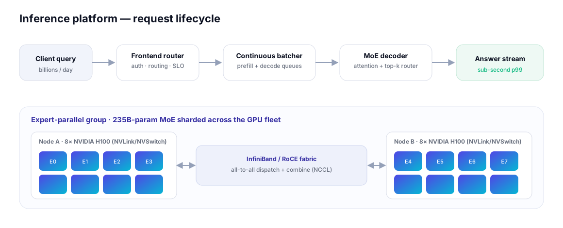Figure 1. The request lifecycle. Compute stages look local; the expert-parallel group hides a network underneath.

A request flows through a frontend router (auth, routing, SLO enforcement), into a continuous batcher that interleaves prefill and decode work to keep GPUs busy, and into the MoE decoder. The decoder runs attention locally, then a top-k gating network selects which experts each token should visit.

Because the 235B parameters do not fit on one GPU, experts are sharded across the fleet using expert parallelism (EP): each GPU owns a subset of experts. When a token is routed to an expert living on a different GPU — which is the common case — its activations must be sent there and the result sent back. That movement is the hidden network we will spend the rest of the article on.

4. Baseline assumptions

Writing down what we expected before measuring is what makes the surprise legible.

We assumed:

1. Attention compute dominates the decode step.
2. GPU utilization is the throughput ceiling — saturate the GPUs and you win.
3. Networking scales linearly — more nodes, proportionally more fabric bandwidth.
4. Expert-routing overhead is small relative to FFN compute.

Every one of these turned out to be wrong at scale, in ways that compounded.

5. Benchmark environment

We built a realistic but hypothetical test bed:

The workload matters: answer generation is decode-heavy. Decode emits one token at a time, so each step moves small tensors very frequently. Hold that thought — it is the crux of the root cause.

6. First benchmark results

We scaled the fleet with the model and traffic mix held constant and measured relative throughput:

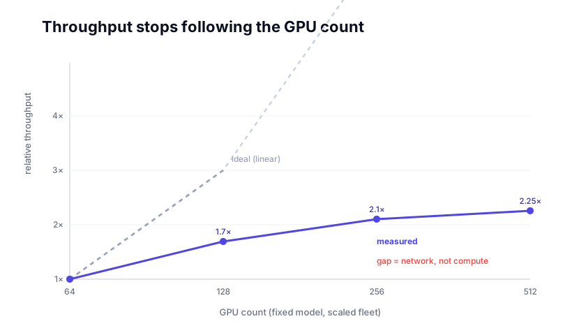Figure 2. Throughput decouples from GPU count. The widening gap is the cost of communication, not a shortage of compute.

The curve flattens hard. By 512 GPUs we were paying for 8× the hardware to get a little over 2× the work. GPU utilization counters, meanwhile, looked fine on average — which is exactly how this class of bug hides.

7. Investigation phase

7.1 GPU analysis

We started where the assumptions pointed. Using Nsight Systems to capture a timeline and DCGM for fleet-wide counters:

# Per-rank timeline with NVTX ranges and NCCL/cuDNN traces
nsys profile -t cuda,nvtx,nccl -o decode_step \
  --capture-range=cudaProfilerApi python serve_decode.py

The kernels were healthy: attention and FFN GEMMs hit expected SM occupancy, HBM bandwidth was nowhere near saturated, and there were no obvious stalls inside the compute kernels. Average SM utilization looked acceptable — but the timeline told a different story: long, recurring gaps between kernels, aligned across ranks. The GPUs were synchronized in their idleness.

7.2 Router analysis

Next we instrumented the gating network and logged per-expert token counts. Routing was not uniform. With learned top-2 gating, a handful of experts attracted disproportionate traffic:

expert_load (tokens/step, normalized):
  E0:1.0  E1:0.9  ...  E17:6.1  ...  E63:0.4

Expert 17 was receiving roughly 6× the average load. Token routing in trained MoE models is rarely balanced in practice; popularity is data-dependent and drifts over time. A hot expert means a hot destination on the network.

7.3 Network analysis

The aligned idle gaps plus a hot destination pointed straight at the fabric. We read InfiniBand port and switch counters and NCCL transport stats:

NCCL_DEBUG=INFO NCCL_DEBUG_SUBSYS=NET python serve_decode.py
perfquery -x            # IB port counters: xmit/rcv data, wait, congestion

The fabric showed the signature of congestion: rising switch-buffer occupancy, PFC pause frames (RoCE) / congestion-control throttling (InfiniBand), and ECN marks concentrated on the links feeding the hot experts. The story had begun.

8. The hidden cost of MoE

The decode loop most engineers picture is compute: attention → FFN → next token. The loop that actually governs throughput is communication:

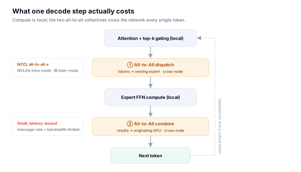Figure 3. Every decode step contains two network collectives — dispatch and combine — repeated for every output token.

Each decode step performs two all-to-all collectives:

1. Dispatch — every GPU sends each token to the GPU that owns its selected expert.
2. Combine — every GPU sends the expert outputs back to the token’s origin.

In NVIDIA’s stack these are typically realized as a grouped sequence of ncclSend/ncclRecv calls (an all-to-all-v pattern) so that each rank can send different amounts to different peers — because, as we saw, the distribution is uneven. Intra-node hops ride NVLink/NVSwitch; inter-node hops ride InfiniBand with GPUDirect RDMA, so the NIC reads and writes GPU memory directly without bouncing through the CPU.

The critical property: in decode, each of these transfers is small (one token’s hidden state per expert) but extremely frequent (twice per token). That makes the all-to-all latency- and message-rate-bound, not bandwidth-bound. You can have terabytes per second of fabric bandwidth sitting idle while throughput collapses, because the limiter is how many small messages per second the fabric and NICs can push — and how long the slowest one takes.

9. Why expert parallelism creates network hotspots

Four effects compound:

Hot experts. Learned routing concentrates traffic on a few experts. Their host GPUs become network destinations far above the average.

Incast. In a single step, many source GPUs send to the same hot expert at the same time. Their flows converge on one switch egress port, overflowing its buffer.

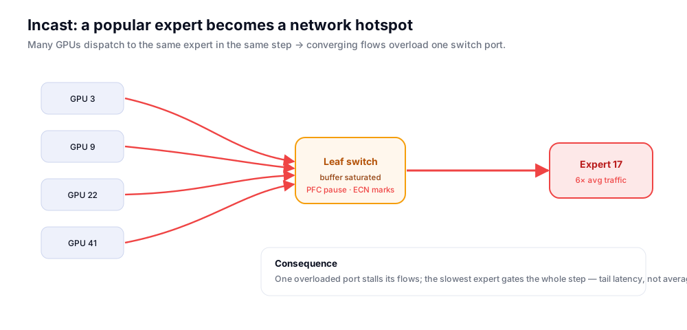Figure 4. Incast: synchronized convergence onto a popular expert saturates a single port, triggering pause/ECN and stalling its senders.

Collective amplification. One routing decision per token fans out into many small transfers across the fabric. Sparse routing turns a compute choice into a communication storm.

Tail latency dominance. A collective is a barrier: the step cannot finish until every transfer completes. One congested port — the slowest expert’s link — gates the entire step. This is why average utilization looked healthy while throughput suffered: the tail, not the mean, sets the pace.

10. Scaling analysis

Zoom out and the geometry gets worse. A flat all-to-all over N GPUs creates on the order of N² small inter-node flows. As N grows:

• At ~100 GPUs, NVLink keeps most traffic node-local; the fabric copes.
• At ~1,000 GPUs, east-west (server-to-server) traffic dominates and spine-leaf pressure becomes the limiter; per-flow bandwidth shrinks as flows multiply.
• At ~10,000 GPUs, locality and topology are the design. Without rack-/rail-aware placement, the bisection bandwidth and switch buffering simply cannot absorb a synchronized N² incast.

The takeaway: beyond a node, throughput is a function of the network topology and the traffic’s locality, not of the GPU count.

11. Mitigations and tradeoffs

There is no single fix. We treated this as a portfolio of changes, each a tradeoff.

Topology-aware expert placement. Place frequently co-activated experts within the same NVLink island so their traffic never touches the fabric. Pro: removes inter-node hops for the hottest paths. Con: placement must track drifting routing distributions; stale placement decays.

Expert replication for hot experts. Replicate the few popular experts across nodes and load-balance across replicas to break the incast. Pro: directly attacks the hotspot. Con: costs memory and adds a consistency/ routing-decision surface.

Hierarchical all-to-all. Aggregate token transfers within a node over NVLink, do a single fat inter-node exchange over InfiniBand, then scatter within the destination node — instead of every GPU talking to every remote GPU directly.

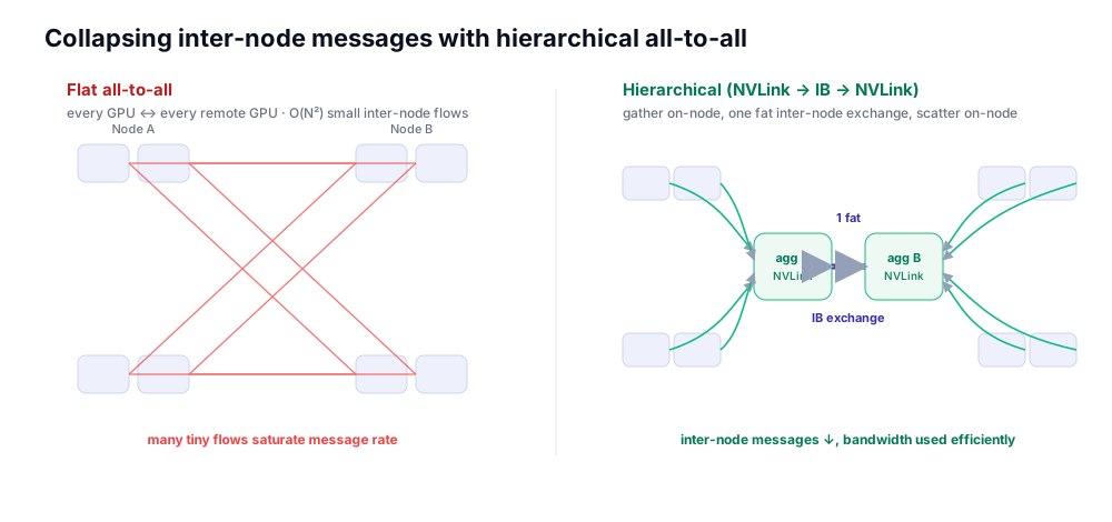Figure 5. Hierarchical all-to-all collapses many tiny inter-node messages into few large ones, trading message rate for bandwidth — the right trade for a fabric that is message-rate-bound.

Pro: converts a message-rate problem into a bandwidth problem the fabric is good at; libraries such as NVSHMEM-based dispatch and modern expert-parallel comm kernels exploit exactly this. Con: added kernel complexity and an extra on-node staging step.

Topology-aware / adaptive routing in the fabric. Enable InfiniBand adaptive routing and tune congestion control (DCQCN/ECN/PFC for RoCE) so converging flows spread across paths rather than piling onto one. Pro: mitigates incast without code changes. Con: tuning is workload-specific and can interact badly with bursty traffic if misconfigured.

Rail-optimized network design. Home each GPU’s NIC to its own rail (leaf), so an all-to-all maps onto parallel, independent rails instead of one shared bottleneck. NCCL’s PXN (PCI × NVLink) path keeps traffic rail-local.

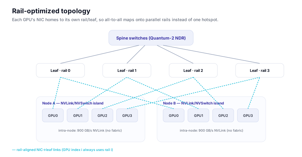Figure 6. Rail-optimized topology. GPU index i always egresses on rail i, so synchronized all-to-all traffic is spread across rails by construction.

Pro: structural — the topology itself prevents a class of hotspot. Con: it is a data-center build decision, hard to retrofit.

Communication-library tuning. NCCL exposes the knobs that decide whether small collectives are fast:

# Prefer low-latency protocols for small decode messages
export NCCL_PROTO=LL128
# Keep transfers on GPUDirect RDMA; never bounce via host
export NCCL_NET_GDR_LEVEL=PHB
# Pin to the rail-local HCA and raise channel count for parallelism
export NCCL_IB_HCA=mlx5
export NCCL_MIN_NCHANNELS=8
# Allow PXN rail-local routing
export NCCL_PXN_DISABLE=0

Pro: large gains for zero hardware cost. Con: values are topology- and shape-specific; the right setting at 128 GPUs may be wrong at 512.

Note on SHARP. NVIDIA’s in-network reduction (SHARP) accelerates reductions such as the all-reduce in tensor-parallel layers, but it does not accelerate the all-to-all that MoE dispatch/combine relies on. It is worth enabling for the parts of the model that reduce — just don’t expect it to fix the MoE hotspot.

12. The bigger insight

In large-scale sparse models, the dominant bottleneck is increasingly communication, not computation. The more we sparsify and distribute a model to save FLOPs, the more we spend on moving activations — and that spending lands on the network.

Said differently: MoE trades compute for communication. That trade is usually a win, but it relocates the bottleneck from a place we instrument well (the GPU) to a place we instrument poorly (the fabric, the tail, the incast). The engineering discipline that matters at scale is communication-aware system design.

13. Implications for future AI systems

The same physics will shape what comes next:

• Trillion-parameter MoE pushes more experts onto more nodes — more all-to-all, more incast, more dependence on topology.
• Agentic systems chain many model calls; their tail latency is a product of per-call tails, so per-call network jitter compounds.
• Distributed KV-cache and memory disaggregation add yet another east-west traffic class competing for the same fabric.
• AI datacenter design increasingly co-designs the model-parallel strategy with the network topology, rather than treating them as separate layers.

14. Production: profiling, fleet, and monitoring

A benchmark fix is not a production fix. Three practices kept the gains in production.

Continuous profiling. Capture periodic per-rank nsys timelines and NVTX-annotated collective spans on a sample of the fleet, so a regression in all-to-all time is caught as a metric, not a customer complaint.

Fleet and topology management. The scheduler is topology-aware: jobs are placed in rail-aligned placement groups, hot-expert replicas are spread across failure domains, and nodes showing fabric degradation are drained rather than left to gate collectives for everyone sharing their step.

Production monitoring. The dashboards that mattered were not GPU utilization — they were network signals:

• per-step all-to-all duration (and its p99), the leading indicator;
• per-expert load skew, to catch routing drift early;
• IB/RoCE congestion counters — PFC pause, ECN marks, switch-buffer occupancy;
• NCCL collective time broken out from compute time via NVTX;
• DCGM fleet telemetry (dcgmi dmon) correlated with the above.

The guiding principle: measure the network and the tail, because the mean will lie to you.

15. Key takeaways

1. MoE shifts the bottleneck from compute to communication. Saving FLOPs costs bytes.
2. Expert popularity creates network hotspots — hot experts plus synchronized incast.
3. GPU utilization hides network inefficiency. Healthy averages, idle tails.
4. Scaling GPUs alone may not raise throughput once you are past one node.
5. Future AI infrastructure must be communication-aware by design — topology, placement, and collectives co-designed with the model.

16. Open questions

• Can expert routing be made topology-aware at inference time without hurting quality?
• Can experts self-balance their load online as traffic drifts?
• Should expert placement be dynamic, migrating hot experts toward demand?
• What is the right benchmark for communication efficiency — a standardized “all-to-all per token at the tail” metric the field could compare against?

References

1. N. Shazeer et al., Outrageously Large Neural Networks: The Sparsely-Gated Mixture-of-Experts Layer, ICLR 2017 (arXiv:1701.06538).
2. D. Lepikhin et al., GShard: Scaling Giant Models with Conditional Computation and Automatic Sharding, 2020 (arXiv:2006.16668).
3. W. Fedus, B. Zoph, N. Shazeer, Switch Transformers: Scaling to Trillion Parameter Models with Simple and Efficient Sparsity, JMLR 2022 (arXiv:2101.03961).
4. S. Rajbhandari et al., DeepSpeed-MoE: Advancing Mixture-of-Experts Inference and Training to Power Next-Generation AI Scale, ICML 2022 (arXiv:2201.05596).
5. C. Hwang et al., Tutel: Adaptive Mixture-of-Experts at Scale, 2022 (arXiv:2206.03382).
6. NVIDIA, NCCL (NVIDIA Collective Communications Library) Documentation — collectives, transports, and environment variables.
7. NVIDIA, NVSHMEM Documentation — GPU-initiated one-sided communication.
8. NVIDIA, Magnum IO and GPUDirect RDMA technical documentation.
9. NVIDIA, NVLink and NVSwitch (H100 / Hopper architecture whitepaper).
10. NVIDIA, Quantum-2 InfiniBand Platform and SHARP In-Network Computing documentation.
11. NVIDIA, DGX SuperPOD Reference Architecture — rail-optimized network design.
12. NVIDIA, Data Center GPU Manager (DCGM) documentation — fleet telemetry.

This is part of an ongoing architecture-study series. Corrections and counterpoints are welcome — the goal is to reason in public about how large AI systems actually behave under load.

The core idea

Treat the provider’s event ID as a unique key and record it the moment you start processing. If you’ve seen it before, acknowledge and stop.

INSERT INTO processed_events (event_id, received_at)
VALUES ($1, now())
ON CONFLICT (event_id) DO NOTHING
RETURNING event_id;

If the RETURNING row is empty, it’s a duplicate — return 200 immediately so the provider stops retrying.

The three stages

1. Verify the signature before trusting anything in the payload.
2. Deduplicate using the insert above, inside the same transaction as your work.
3. Process the side effect, then commit atomically.

The crucial detail is step 2 and 3 sharing one transaction. If processing fails, the dedup row rolls back too, so a legitimate retry can succeed.

Why not just check-then-insert?

Because two concurrent deliveries can both pass the check before either inserts. The ON CONFLICT approach pushes uniqueness into the database, where it’s actually safe under concurrency.

This pattern has handled millions of events for us without a single duplicate-side-effect incident since we shipped it.

The symptom

Dashboards showed a healthy median (~45 ms) but a P99 that spiked unpredictably to nearly a second. Tail latency like this almost never comes from CPU; it comes from waiting — locks, queues, or pools.

Finding the bottleneck

We added per-request spans around three stages: auth, query planning, and the database call. The data was unambiguous:

The database itself was fast. Requests were spending most of their time waiting to acquire a connection from a pool that was sized for average load, not peak.

The fix

Three changes, in order of impact:

1. Right-sized the pool based on peak_concurrency × avg_hold_time, not a guessed number.
2. Added a short acquire timeout so a saturated pool fails fast instead of queueing.
3. Made slow queries observable with a log line above 100 ms.

pool = ConnectionPool(
    min_size=10,
    max_size=64,          # was 20
    timeout=0.25,         # fail fast instead of queueing
)

Results

P99 dropped from 820 ms to 320 ms within an hour of deploy — and stayed flat through the next traffic peak.

No new servers, no query rewrites. The lesson we keep relearning: tail latency is usually a queueing problem, not a compute problem.